Predictors of a regression model for power simulation

Power simulation for regression starts with the question if one should draw the values for the predictors “inside” or “outside” of the power simulation. There is a reason why Florian gives a regression example where the predictor is dose of medication and has therefore fixed values (Wickelmaier 2026, sec. 4). But often we have predictors that can take all kinds of values and we think about these predictors in terms of also being drawn from a distribution. If we draw the predictor in each iteration of a power simulation, we are adding additional variance that the regression model does not account for. Where does this variance go? We will stick to simple regression here.

Drawing values for a predictor once

We will assume that values for our predictor come from a normal distribution. Since I am making this point without any context, let’s just assume a standard normal distribution.

set.seed(1238)

n <- 20
x <- rnorm(n, mean = 0, sd = 1)

We have now drawn our predictor and will use this in a power simulation. Next, we need to specify additional parameters for the simple regression model

\[ y = \beta_0 + \beta_1 x + \varepsilon\] with \(\varepsilon \sim N(0, \sigma^2_\varepsilon)\).

beta <- c(beta0 = 1, beta1 = .5)
se <- 1

We will now run a power simulation to find out how many participants we need to find an effect of \(\beta_1 = 0.5\).

pval <- replicate(2000, {
  y <- beta[1] + beta[2] * x + rnorm(n, mean = 0, sd = se)
  m0 <- lm(y ~ 1)
  m1 <- lm(y ~ x)
  anova(m0, m1)[2, "Pr(>F)"]
  }
)

mean(pval < 0.05)

[1] 0.458

This results in a power that is not sufficient, yet, so let us adjust our N and rerun it.

n <- 25
x <- rnorm(n, mean = 0, sd = 1)

pval <- replicate(2000, {
  y <- beta[1] + beta[2] * x + rnorm(n, mean = 0, sd = se)
  m0 <- lm(y ~ 1)
  m1 <- lm(y ~ x)
  anova(m0, m1)[2, "Pr(>F)"]
  }
)

mean(pval < 0.05)

[1] 0.7965

OK, this looks good. So we need to collect 25 subjects, right? Looks like the power increased quite a bit for just 5 more subjects. Let’s make sure and rerun it.

set.seed(12)

n <- 25
x <- rnorm(n, mean = 0, sd = 1)

pval <- replicate(2000, {
  y <- beta[1] + beta[2] * x + rnorm(n, mean = 0, sd = se)
  m0 <- lm(y ~ 1)
  m1 <- lm(y ~ x)
  anova(m0, m1)[2, "Pr(>F)"]
  }
)

mean(pval < 0.05)

[1] 0.6125

Obviously, the power is strongly influenced by our predictor and what values it takes. What happens when we draw the predictor within each iteration of the power simulation? And are there differences in parameter recovery for these two approaches?

Drawing values for the predictor in each iteration

set.seed(1450)

n <- 25

pval <- replicate(2000, {
  # Draw predictor
  x <- rnorm(n, mean = 0, sd = 1)
  # Simulate dependent variable
  y <- beta[1] + beta[2] * x + rnorm(n, mean = 0, sd = se)
  m0 <- lm(y ~ 1)
  m1 <- lm(y ~ x)
  anova(m0, m1)[2, "Pr(>F)"]
  }
)

mean(pval < 0.05)

[1] 0.6365

With this approach we see that N = 25 is not enough to find our effect with a power of 80%.

n <- 37

pval <- replicate(2000, {
  # Draw predictor
  x <- rnorm(n, mean = 0, sd = 1)
  # Simulate dependent variable
  y <- beta[1] + beta[2] * x + rnorm(n, mean = 0, sd = se)
  m0 <- lm(y ~ 1)
  m1 <- lm(y ~ x)
  anova(m0, m1)[2, "Pr(>F)"]
  }
)

mean(pval < 0.05)

[1] 0.81

Power estimation with this approach is more stable than when we draw the predictor only once. But what does this mean for parameter recovery?

Parameter recovery

Drawing values for a predictor once

n <- 200

# Draw predictor
x <- rnorm(n, mean = 0, sd = 1)

out <- replicate(2000, {
  # Simulate dependent variable
  y <- beta[1] + beta[2] * x + rnorm(n, mean = 0, sd = se)
  m <- lm(y ~ x)
  c(coef(m), sigma = sigma(m))
  }
)

boxplot(t(out))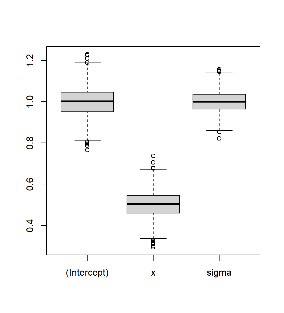

rowMeans(out)

(Intercept)           x       sigma 
  0.9986695   0.5022547   0.9995984

Drawing values for the predictor in each iteration

n <- 200

out <- replicate(2000, {
  # Draw predictor
  x <- rnorm(n, mean = 0, sd = 1)
  # Simulate dependent variable
  y <- beta[1] + beta[2] * x + rnorm(n, mean = 0, sd = se)
  m <- lm(y ~ x)
  c(coef(m), sigma = sigma(m))
  }
)

boxplot(t(out))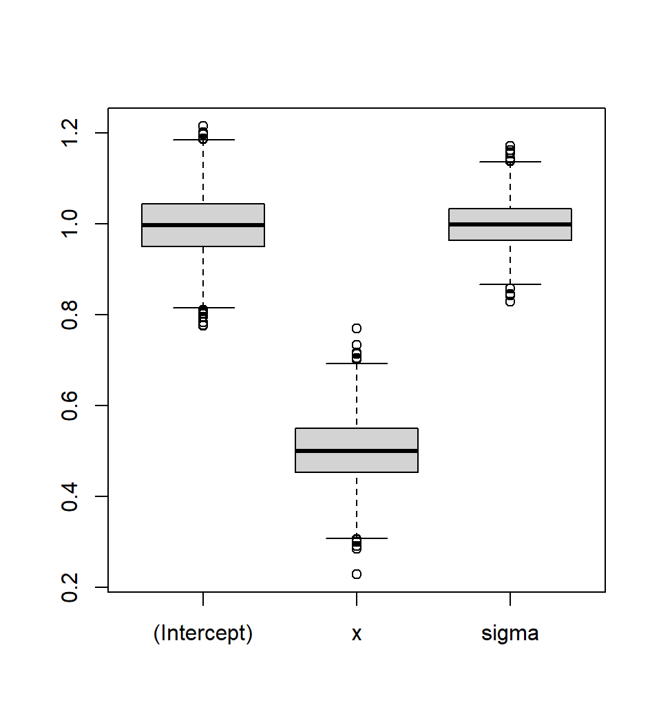

rowMeans(out)

(Intercept)           x       sigma 
  0.9983379   0.5017602   0.9996439

Interestingly, there is no difference in parameter recovery. That is actually not what I expected.

Conlusions

But that makes the conclusion easy. Then I would recommend drawing the predictor in each iteration of the power simulation since this makes the power estimation much more stable. This is, of course, the easiest version of this simulation. What happens if one draws more than one predictor or if the predictors are correlated?

Session info

sessionInfo()

R version 4.6.1 (2026-06-24 ucrt)
Platform: x86_64-w64-mingw32/x64
Running under: Windows 11 x64 (build 26100)

Matrix products: default
  LAPACK version 3.12.1

locale:
[1] LC_COLLATE=German_Germany.utf8  LC_CTYPE=German_Germany.utf8   
[3] LC_MONETARY=German_Germany.utf8 LC_NUMERIC=C                   
[5] LC_TIME=German_Germany.utf8    

time zone: Europe/Berlin
tzcode source: internal

attached base packages:
[1] stats     graphics  grDevices utils     datasets  methods   base     

loaded via a namespace (and not attached):
 [1] htmlwidgets_1.6.4 compiler_4.6.1    fastmap_1.2.0     cli_3.6.6        
 [5] tools_4.6.1       htmltools_0.5.9   otel_0.2.0        yaml_2.3.12      
 [9] rmarkdown_2.32    knitr_1.52        jsonlite_2.0.0    xfun_0.62        
[13] digest_0.6.39     rlang_1.3.0       evaluate_1.0.5

References

Wickelmaier, F. 2026. “Simulating the Power of Statistical Tests: A Collection of R Examples.” ArXiv. https://doi.org/10.48550/arXiv.2110.09836.