Question from statistics consulting

A few weeks ago, we met to talk about a power analysis for my pre/post study. Now, I want to add a second delayed post-test assessment one week later. Does this change my power simulation?

Short answer: Yes, quite dramatically. ;)

Power simulation for ANCOVA (two time points)

This power simulation for the original pre/post design assumed that the data will be analyzed with an ANCOVA model (based on the paper by Vickers and Altman 2001). This is the original power simulation based on values found for previous data collected by this PhD student.

n <- 87

# Draw plausible pre values and setup data frame
dat <- data.frame(
  pre = rnorm(n, mean = 12.5, sd = 3.5),
  grp = factor(rep(1:3, each = n/3), labels = c("g1", "g2", "g3"))
)

# Specify the minimum relevant average treatment effects and set the remaining
# parameters to plausible values

# mu = mean learning outcome (expected pre-post effect in reference group)
# b  = slope between pre and post values
# a2 = expected difference between group 2 and group 1
# a3 = expected difference between group 3 and group 1
# se = sigma of ANCOVA model

beta <- c(mu = 3, b = .7, a2 = 1.5, a3 = 3)
means <- model.matrix(~ pre + grp, dat) %*% beta
se <- 2

# Estimate power
pval <- replicate(2000, {
  post <- means + rnorm(n, sd = se)
  m <- lm(post ~ pre + grp, dat)
  summary(m)$coef["grpg2", "Pr(>|t|)"]
})

mean(pval < 0.05)

[1] 0.8015

I will not go into detail, why this is the appropriate analysis for this design. Maybe this will become another post at some point. Read the paper by Vickers and Altman (2001) in the meantime.

Power simulation for mixed-effects model (three time points)

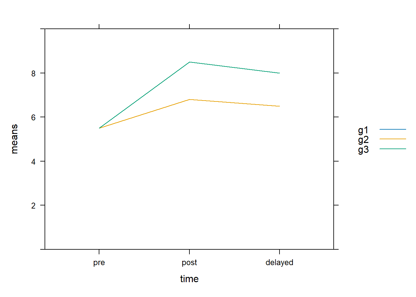
Unfortunately, when we add another time point into the mix, we now have to switch the analysis to a mixed-effects model with a group x time interaction. It was also much harder for the PhD student to term her hypothesis in terms of model parameters. So, I made her draw the expected pattern and add mean values to the plot. This is what she came up with.

n <- 3

design <- data.frame(id = factor(rep(1:n, each = 3)),
                  time = factor(rep(c("pre", "post", "delayed"), times = n),
                                levels = c("pre", "post", "delayed")),
                  grp = factor(rep(1:3, each = 3, times = n / 3),
                               labels = c("g1", "g2", "g3"))
)


means <- c(5.5, 6.8, 6.5, 5.5, 6.8, 6.5, 5.5, 8.5, 8)

lattice::xyplot(means ~ time, data = design, groups = grp,
                type = "a",
                ylim = 0:10,
                auto.key = TRUE)

We can now use these means and the “design” data frame to calculate the fixed model parameters with

\[ \mathbf{\beta} = X^{-1} \mathbf{\mu} \]

mm <- model.matrix(~ grp * time, data = design)
(beta <- as.vector(solve(mm) %*% means))

[1] 5.5 0.0 0.0 1.3 1.0 0.0 1.7 0.0 1.5

Now, we still need the variance terms for the random effects. For simplicity reasons, we still stick to a random intercept model here. So we need to specify a residual variance and a person variance.

sp <- 1.5
se <- 2

The power simulation then looks something like this.

library("lme4")

n <- 120

dat <- data.frame(id = factor(rep(1:n, each = 3)),
                  time = factor(rep(c("pre", "post", "delayed"), times = n),
                                levels = c("pre", "post", "delayed")),
                  grp = factor(rep(1:3, each = 3, times = n / 3),
                               labels = c("g1", "g2", "g3"))
)


mm <- model.matrix(~ grp * time, data = dat)
means <- as.vector(mm %*% beta)


pval <- replicate(1000, {
  y <- means +                                        # structural part
       rep(rnorm(n, mean = 0, sd = sp), each = 3) +   # person effect
       rnorm(n * 3, mean = 0, sd = se)                # random error
  m0 <- lmer(y ~ grp + time + (1 | id), data = dat, REML = FALSE)
  m1 <- lmer(y ~ grp * time + (1 | id), data = dat, REML = FALSE)
  # Likelihood-Ratio-Test
  anova(m0, m1)["m1", "Pr(>Chisq)"]
  }
)

mean(pval < 0.05)

[1] 0.774

For more examples how to run power simulations in R see Wickelmaier (2026).

Session info

sessionInfo()

R version 4.6.1 (2026-06-24 ucrt)
Platform: x86_64-w64-mingw32/x64
Running under: Windows 11 x64 (build 26100)

Matrix products: default
  LAPACK version 3.12.1

locale:
[1] LC_COLLATE=German_Germany.utf8  LC_CTYPE=German_Germany.utf8   
[3] LC_MONETARY=German_Germany.utf8 LC_NUMERIC=C                   
[5] LC_TIME=German_Germany.utf8    

time zone: Europe/Berlin
tzcode source: internal

attached base packages:
[1] stats     graphics  grDevices utils     datasets  methods   base     

other attached packages:
[1] lme4_2.1-0   Matrix_1.7-6

loaded via a namespace (and not attached):
 [1] digest_0.6.39     fastmap_1.2.0     xfun_0.62         lattice_0.23-1   
 [5] splines_4.6.1     knitr_1.52        htmltools_0.5.9   rmarkdown_2.32   
 [9] Rdpack_2.6.6      cli_3.6.6         nloptr_2.2.1      grid_4.6.1       
[13] reformulas_0.4.4  compiler_4.6.1    rbibutils_2.4.1   boot_1.3-32      
[17] tools_4.6.1       nlme_3.1-171      minqa_1.2.8       evaluate_1.0.5   
[21] Rcpp_1.1.2        yaml_2.3.12       otel_0.2.0        rlang_1.3.0      
[25] jsonlite_2.0.0    htmlwidgets_1.6.4 MASS_7.3-66

References

Vickers, A. J., and D. G. Altman. 2001. “Analysing Controlled Trials with Baseline and Follow up Measurements.” British Medical Journal 323 (7321): 1123–24. https://doi.org/10.1136/bmj.323.7321.1123.

Wickelmaier, F. 2026. “Simulating the Power of Statistical Tests: A Collection of R Examples.” ArXiv. https://doi.org/10.48550/arXiv.2110.09836.