library("lattice")
library("metafor")Question from statistics consulting
I want to report an aggregated effect size over several of my studies. Should I use a meta-analysis for that or is there a better way?
Shortly before I started working as a statistical consultant, Daniel Lakens gave a workshop at our institute on “How to better your inference”. Unfortunately, I missed it, but a lot of the doctoral students at our institute were greatly influenced by this workshop. My guess is that this led to the practice of “internal meta-analyses” for a lot of the PhD projects (Lakens mentions it here). I was suprised, when I was confronted with this practice for the first time. It seemed silly to me to do a meta-analysis for studies where one has full access to the complete data (since those studies were conducted by oneself).
In order to get a clearer idea about this practice, I ran a small simulation where I simulated data for several studies with different N with the same underlying effect and then ran a meta-analysis with metafor and a simple regression model where I added a variable study as a covariate.
Data simulation
set.seed(1109)

# Set effect coding to get the treatment effect for an "average" study
options(contrasts = c("contr.sum", "contr.poly"))

# Simulate data for 10 studies
n <- c(20, 50, 30, 26, 10, 20, 30, 100, 20, 46)
mu <- 1                                          # mean in control group
d_true <- 1                                      # "true" effect
What excatly did we do here? We assume that we conducted 10 different studies with a different number of participants ranging from 10 to 100. We have two groups: Control (ctr) vs. Treatment (trt) and want to compare the treatment effect (the difference in the DV between the two groups). We set the mean in the control group to \(\mu = 1\) and assume a true treatment effect \(\delta_{true} = 1\).
sd <- 1The next thing we need to decide on is the variation in the data. We set the varianz in the data to \(\sigma = 1\).
d_obs <- rnorm(length(n), mean = d_true, sd = 2 / sqrt(n))Next we draw the effect sizes for each of the studies. We assume that they come from a normal distribution with \(N(\mu = 1, \sigma = \frac{2}{\sqrt{n}})\). Doing it like this is in line with a fixed-effect model for meta-analysis. Since we are in the “theoretical” mindframe that all studies originated in the same lab under very similar conditions this might be a reasonable choice? Go ahead and adjust the simulation so the underlying model corresponds to a random-effects model for meta-analysis. Do the results change? (I did not try it.)
I must admit that I have no good idea how to draw the effect sizes for the study. I decided to weigh the variance by \(\frac{1}{\sqrt{n}}\) so that for bigger \(n\) the variance is smaller and, therefore, the probability to draw a value closer to the “true” value is higher. I added this later on. When you leave this out and draw all effect sizes with same variance, then the meta-analysis has a much wider confidence intervall for the estimate of the treatment effect. I guess that makes sense. Well, I guess doing it with a weighted variance is in line with a frequentist view and also with the underlying assumptions for meta-analysis.
dat_list <- list()

for (i in 1:10) {
  dat0 <- data.frame(id = factor(1:n[i]),
                     group = factor(rep(c("ctr", "trt"), each = n[i] / 2),
                                    levels = c("trt", "ctr")),
                     resp = c(rnorm(n[i] / 2, mean = mu, sd = sd),
                              rnorm(n[i] / 2, mean = mu + d_obs[i], sd = sd)),
                     n = n[i],
                     study = factor(paste0("study", sprintf("%02d", i))))
  dat_list[[i]] <- dat0
}

rm(dat0)

# Integrate into one dataframe
dat_all <- do.call("rbind", dat_list)

bwplot(resp ~ factor(group, levels = c("ctr", "trt")) | study, data = dat_all,
       layout = c(5, 2))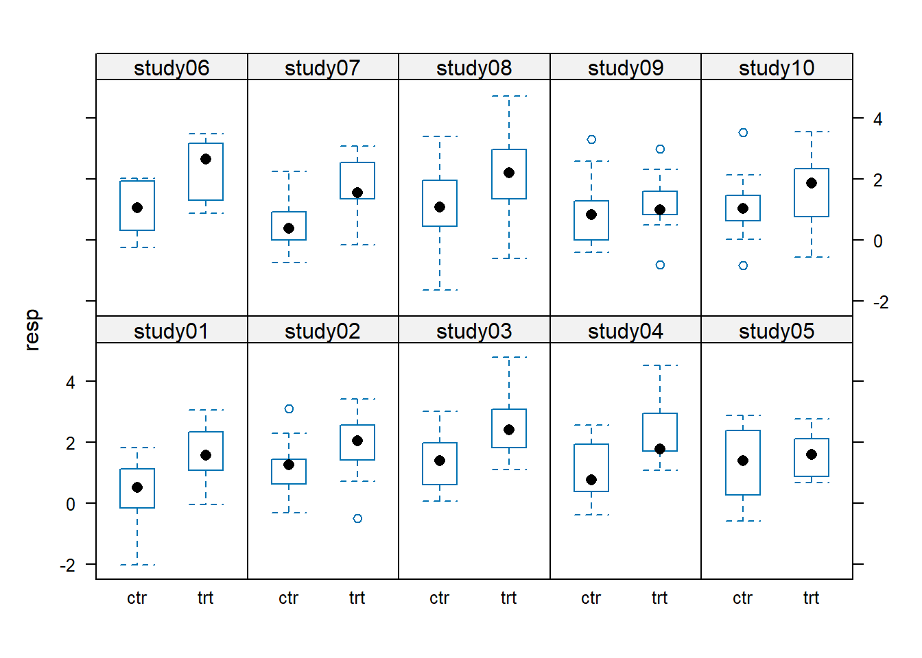
Analyze the data
# Analyzing all data in one model
m1 <- lm(resp ~ group, data = dat_all)
summary(m1)
Call:
lm(formula = resp ~ group, data = dat_all)

Residuals:
     Min       1Q   Median       3Q      Max
-3.04447 -0.70303  0.01982  0.79411  2.80768

Coefficients:
            Estimate Std. Error t value Pr(>|t|)
(Intercept)   1.4982     0.0539  27.798   <2e-16 ***
group1        0.4772     0.0539   8.854   <2e-16 ***
---
Signif. codes:  0 '***' 0.001 '**' 0.01 '*' 0.05 '.' 0.1 ' ' 1

Residual standard error: 1.011 on 350 degrees of freedom
Multiple R-squared:  0.183, Adjusted R-squared:  0.1806
F-statistic: 78.39 on 1 and 350 DF,  p-value: < 2.2e-16
# Estimated treatment effect
coef(m1)["group1"] * 2 group1
0.9543521 This ignores completely that the data were collected in different studies. Let us add a covariate study to the model and see what the estimated treatment effect for an “average” study looks like.
# Adding study as a covariate to the model
m2 <- lm(resp ~ group + study, data = dat_all)
summary(m2)
Call:
lm(formula = resp ~ group + study, data = dat_all)
Residuals:
Min 1Q Median 3Q Max
-2.78958 -0.70356 0.00348 0.72203 2.72573
Coefficients:
Estimate Std. Error t value Pr(>|t|)
(Intercept) 1.44624 0.06319 22.888 < 2e-16 ***
group1 0.47718 0.05280 9.038 < 2e-16 ***
study1 -0.44367 0.20795 -2.133 0.03360 *
study2 0.10850 0.14033 0.773 0.43997
study3 0.49978 0.17367 2.878 0.00426 **
study4 0.24583 0.18490 1.330 0.18455
study5 -0.01158 0.28722 -0.040 0.96786
study6 0.22640 0.20795 1.089 0.27706
study7 -0.31949 0.17367 -1.840 0.06669 .
study8 0.17633 0.10883 1.620 0.10609
study9 -0.38748 0.20795 -1.863 0.06328 .
---
Signif. codes: 0 '***' 0.001 '**' 0.01 '*' 0.05 '.' 0.1 ' ' 1
Residual standard error: 0.9906 on 341 degrees of freedom
Multiple R-squared: 0.2361, Adjusted R-squared: 0.2137
F-statistic: 10.54 on 10 and 341 DF, p-value: 1.442e-15# Estimated treatment effect
coef(m2)["group1"] * 2 group1
0.9543521 The effect is exactly the same… Is this always true? Why would I even add the covariate then?
# Doing a metaanalysis on these data
datm <- aggregate(resp ~ study + group, data = dat_all, FUN = mean)
datm$sd <- aggregate(resp ~ study + group, data = dat_all, FUN = "sd")[, 3]
datm$n <- aggregate(resp ~ study + group, data = dat_all, FUN = "length")[, 3]
es <- escalc("MD",
m1i = datm$resp[datm$group == "trt"],
m2i = datm$resp[datm$group == "ctr"],
sd1i = datm$sd[datm$group == "trt"],
sd2i = datm$sd[datm$group == "ctr"],
n1i = datm$n[datm$group == "trt"],
n2i = datm$n[datm$group == "ctr"])
res <- rma(yi, vi, data=es)
forest(res)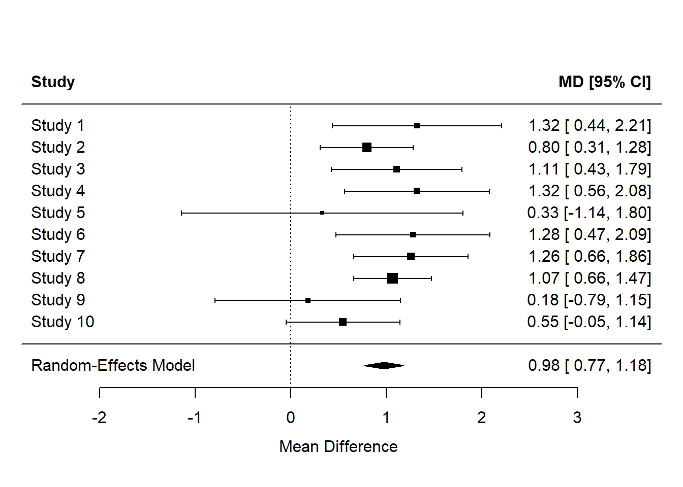
Conclusions
# Compare true and estimated treatment effects
est <- c(d_true, res$beta, coef(m2)[2] * 2)
cilb <- c(NA, res$ci.lb, confint(m2)[2, 1] * 2)
ciub <- c(NA, res$ci.ub, confint(m2)[2, 2] * 2)
cbind(est, cilb, ciub) est cilb ciub
1.0000000 NA NA
0.9767077 0.7728563 1.180559
group1 0.9543521 0.7466444 1.162060par(mai = c(.6, .7, .1, .1), mgp = c(2.4, 1, 0))
plot(est, axes = F, ylim = c(-1,3), pch = 16, cex = 2, xlab = "",
ylab = "Mean difference")
arrows(1:3, cilb, 1:3, ciub, code = 3, length = .05, angle = 90)
axis(1, at = 1:3, labels = c("true", "ma", "lm"))
axis(2)
abline(h = est[1], lty = 3)
abline(h = 0, lty = 3, col = "red")
box()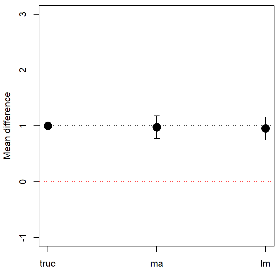
The results (for this one draw of 10 studies!) show that the meta-analysis and the regression model with study as covariate show pretty similar estimates for the treatment effect. The confidence intervalls look also similar. I guess, the main advantage of the meta-analysis is the beautiful plot that you can create with metafor out of the box… I am still not sure why we even need the covariate in this. Guess, I have to think about this some more.
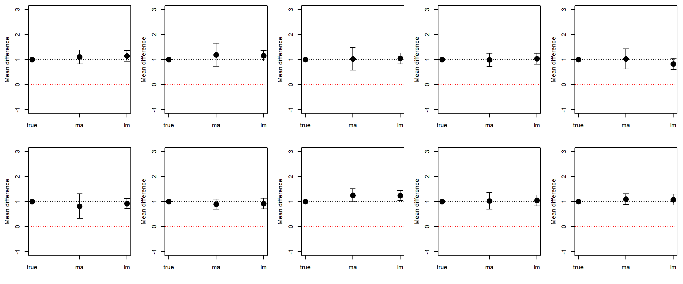
Do it ten times for 10 studies
I repeated the code from above ten times to get an idea how stable the results are. Here are the plots. Looks like the estimate obtained via meta-analysis is a bit more “uncertain”. Guess, that is a good thing.
Session info
sessionInfo()R version 4.6.1 (2026-06-24 ucrt)
Platform: x86_64-w64-mingw32/x64
Running under: Windows 11 x64 (build 26100)
Matrix products: default
LAPACK version 3.12.1
locale:
[1] LC_COLLATE=German_Germany.utf8 LC_CTYPE=German_Germany.utf8
[3] LC_MONETARY=German_Germany.utf8 LC_NUMERIC=C
[5] LC_TIME=German_Germany.utf8
time zone: Europe/Berlin
tzcode source: internal
attached base packages:
[1] stats graphics grDevices utils datasets methods base
other attached packages:
[1] metafor_5.2-1 numDeriv_2016.8-1.1 metadat_1.6-0
[4] Matrix_1.7-6 lattice_0.23-1
loaded via a namespace (and not attached):
[1] digest_0.6.39 fastmap_1.2.0 xfun_0.62 knitr_1.52
[5] htmltools_0.5.9 rmarkdown_2.32 mathjaxr_2.0-0 cli_3.6.6
[9] grid_4.6.1 compiler_4.6.1 tools_4.6.1 nlme_3.1-171
[13] evaluate_1.0.5 yaml_2.3.12 otel_0.2.0 rlang_1.3.0
[17] jsonlite_2.0.0 htmlwidgets_1.6.4