library("fGarch")

xi <- 2

x <- rsnorm(1000, mean = 0, sd = 1, xi = xi)
hist(x, freq = FALSE, ylim = c(0, .5), border = "white", main = "")
curve(dsnorm(x, xi = xi), -2.5, 4.5, add = TRUE, lwd = 2)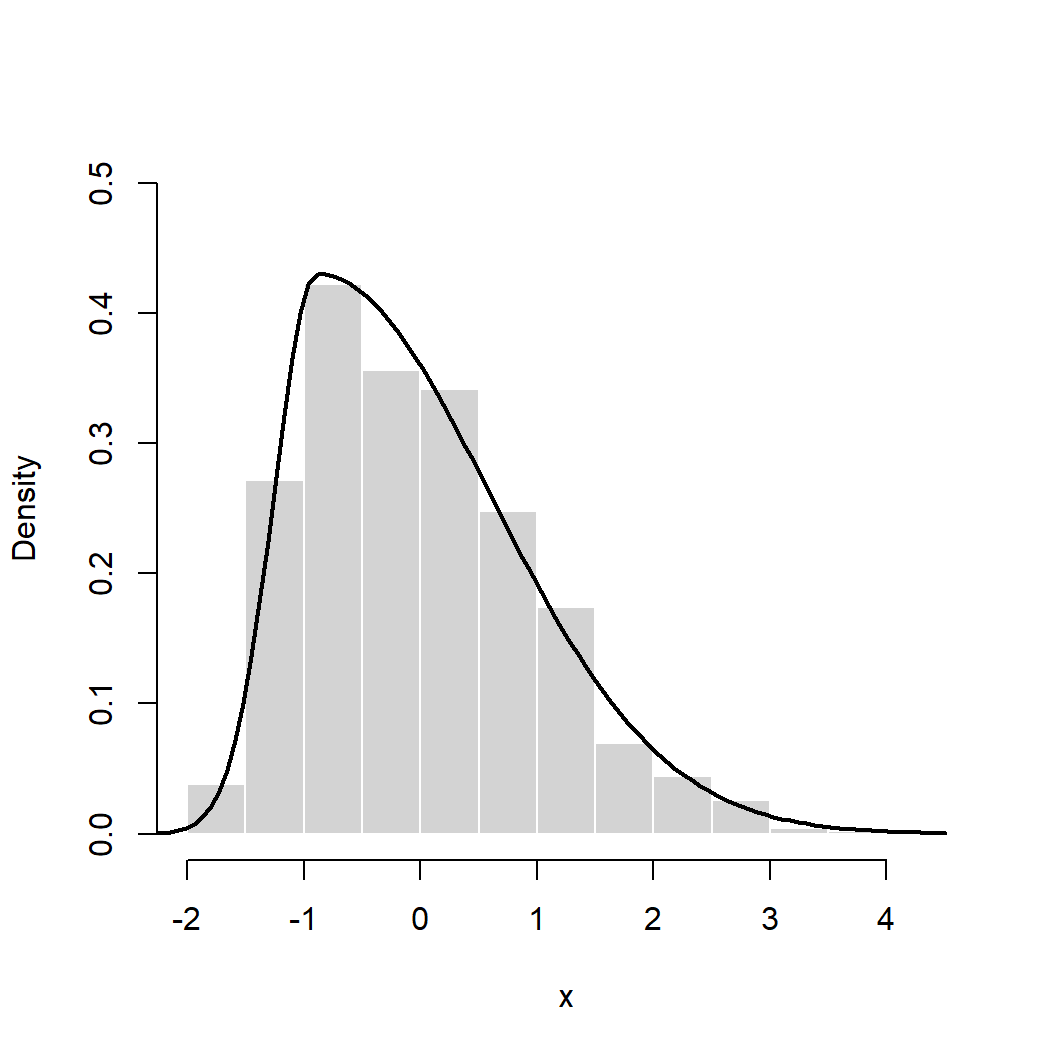
In the era of preregistration and after the replication crisis in psychology (and, of course, other disciplines), I am inclined to use the sentence “No analysis decisions after we have seen the data” quite often during statistical consultations. If you want to read up on this, read the paper by Gelman and Loken.
But this is very different from what most people learned in their statistics courses, where they have been taught to first test, e.g., for variance homogeneity and then decide on an apropriate test: either a t-test or a Welch test, for example. If you want to play around with this, check out this shiny app: https://apps.mathpsy.uni-tuebingen.de/fw/condtest/. It is quite instructive and strongly suggests that one should always perform a Welch test, independently of violations of variance homogeneity.
A common reason for people to seek statistics consultation from me, is that the normality assumption of their data is violated and now they wonder if their planned (and usually preregistered) analysis is still the best choice. Ususally, we are talking analysis of variance or regression here.
Based on the shiny app mentioned above, I thought, I could maybe try out what happens if the normality assumption is violated.
I found an R package that lets you simulate data from a “skew normal distribution” (I guess, that’s an oxymoron, but what the heck): fGarch.
With the function fGarch::rsnorm() we can simulate skewed data. The argument xi controls the extend of the skewness. Let us have a look.
library("fGarch")
xi <- 2
x <- rsnorm(1000, mean = 0, sd = 1, xi = xi)
hist(x, freq = FALSE, ylim = c(0, .5), border = "white", main = "")
curve(dsnorm(x, xi = xi), -2.5, 4.5, add = TRUE, lwd = 2)
The first step in an analysis procedure like this is to decide which test to use when testing for normality. There are many different options. Honestly, I have never given too much thought to this. I learned at some point that most of these tests have bad statistical properties and luckily I was never in s situation where I had to apply these tests. Two common choices are the Kolmogorov-Smirnov test and the Shapiro-Wilk test of normality. Both are available in the stats package in R. I ran a small simulation and was a bit suprised by the results. (I am sure that shows my ignorance on the topic and that there are much better choices for testing normality. However, these are common choices that I regularly encounter in statistics consultation.)
compare_normtest <- function(xi, n_group, test = "Shapiro", all_skewed = TRUE) {
  pval <- replicate(2000, {
    if (all_skewed) {
      resp1 <- rsnorm(n_group, mean = 0, sd = 1, xi = xi)
    } else {
      resp1 <- rsnorm(n_group, mean = 0, sd = 1, xi = 1)
    }
    resp2 <- rsnorm(n_group, mean = 0, sd = 1, xi = xi)
    resp3 <- rsnorm(n_group, mean = 0, sd = 1, xi = xi)
    dat <- data.frame(cond = rep(c("c1", "c2", "c3"), each = n_group),
                      resp = c(resp1, resp2, resp3))
    ifelse(test == "Shapiro",
           shapiro.test(dat$resp)$p.value,
           ks.test(dat$resp, "pnorm", mean = 0, sd = 1)$p.value)
  })
  mean(pval < .05)
}

comb <- expand.grid(xi = c(1, 3, 5),
                    n_group = c(10, 50, 100),
                    test = factor(c("Shapiro", "Kolmogorov-Smirnov")),
                    all_skewed = c(TRUE, FALSE))

comb$pwr <- mapply(compare_normtest, n_group = comb$n_group,
                   xi = comb$xi, test = comb$test, all_skewed = comb$all_skewed)

lattice::xyplot(pwr ~ n_group | factor(all_skewed,
                                       labels = c("one normal group",
                                                  "all groups skewed")) + test,
                data = comb, groups = xi,
                type = c("g", "b"),
                xlab = "N in each group",
                ylab = "Power",
                auto.key = list(space = "top", columns = 3, title = expression(xi)))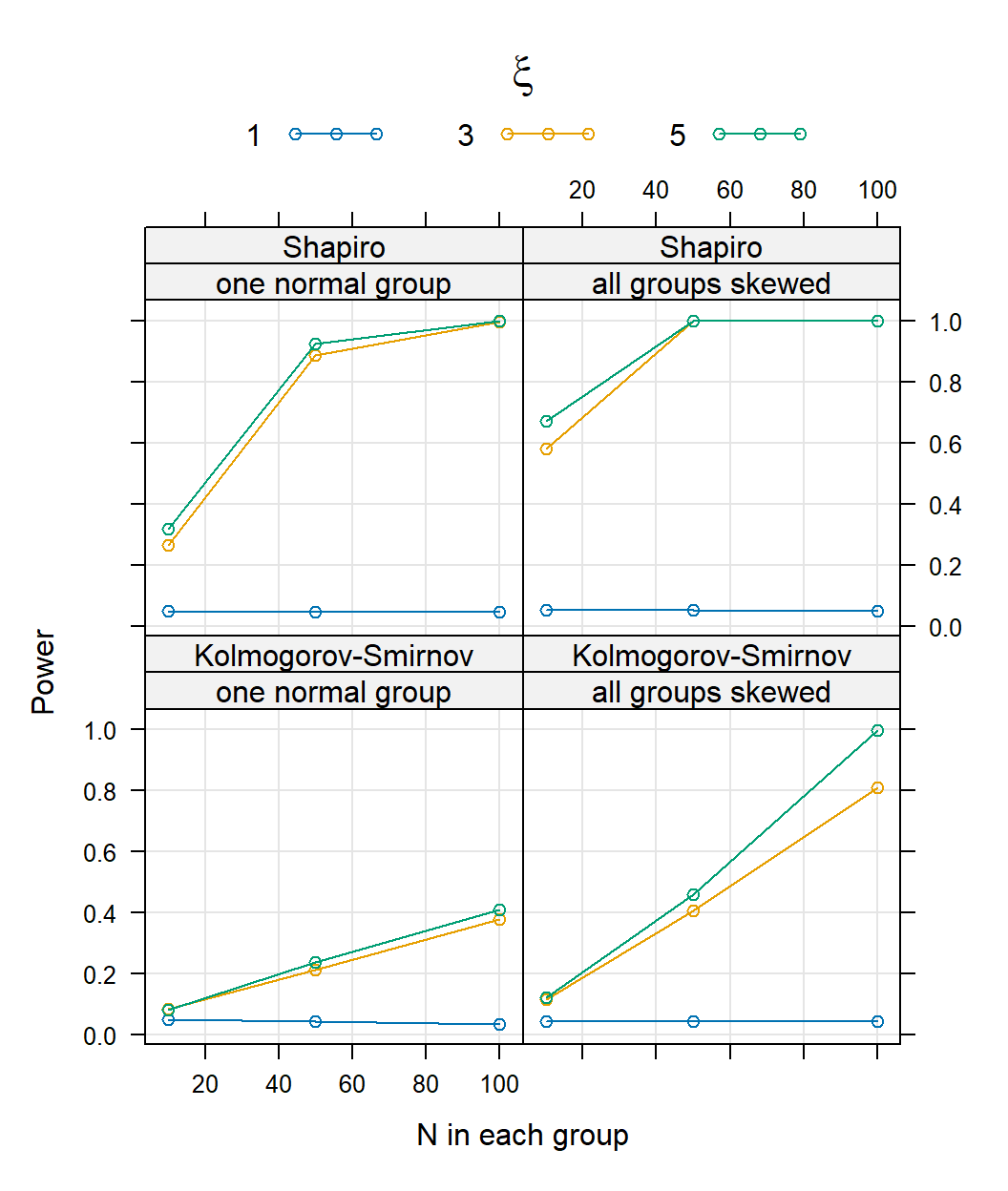
Based on this plot I am inclined to go with the Shapiro test here. But go on and try it out with other tests testing the normality assumption yourself!
Next, I will simulate data for three independent groups. I will simulate data for each of these groups separately, but always assuming the same size of skewness and the same sample size N. I will let \(\xi\) vary from 1 (normal distribution) to 10 (very skewed) and N take the values 10, 100, and 500. To each data set, we will fit an ANOVA with aov(), a Kruskal-Wallis rank sum test with kruskal.test() which is a nonparametric test meaning its only assumption is that the data are continuous but not which distribution it follows. Additionally, we will first test for normality of the data and then decide if we do an ANOVA or a Kruskal-Wallis rank sum test based on the results. Hence, we condition our analysis on the data.
compare_parametric <- function(xi, n_group = 20, test, all_skewed = TRUE) {
  pval <- replicate(1000, {
    if (all_skewed) {
      resp1 <- rsnorm(n_group, mean = 0, sd = 1, xi = xi)
    } else {
      resp1 <- rsnorm(n_group, mean = 0, sd = 1, xi = 1)
    }
    resp2 <- rsnorm(n_group, mean = 0, sd = 1, xi = xi)
    resp3 <- rsnorm(n_group, mean = 0, sd = 1, xi = xi)

    dat <- data.frame(cond = factor(rep(c("c1", "c2", "c2"), each = n_group)),
                      resp = c(resp1, resp2, resp3))
    if (test == "ANOVA") {
      anova(lm(resp ~ cond, dat))["cond", "Pr(>F)"]
    } else if (test == "Kruskal") {
      kruskal.test(resp ~ cond, dat)$p.value
    } else {
      ifelse(shapiro.test(dat$resp)$p.value >= .05,
             anova(lm(resp ~ cond, dat))["cond", "Pr(>F)"],
             kruskal.test(resp ~ cond, dat)$p.value)
    }
  })
  mean(pval < .05)
}

comb <- expand.grid(xi = 1:10, n_group = c(10, 100, 500),
                    test = c("ANOVA", "Kruskal", "Conditioned"),
                    all_skewed = c(TRUE, FALSE))

comb$pwr <- mapply(compare_parametric,
                   xi = comb$xi,
                   n_group = comb$n_group,
                   test = comb$test,
                   all_skewed = comb$all_skewed)

lattice::xyplot(pwr ~ xi | factor(all_skewed,
                                  labels = c("one normal group",
                                             "all groups skewed")) +
                           factor(n_group,
                                  labels = paste("N =", unique(n_group))),
                data = comb,
                groups = test,
                type = c("g", "b"),
                xlab = expression(xi),
                ylab = "Type I Error Rate",
                ylim = c(0, 0.5),
                auto.key = list(space = "top", columns = 3,
                                title = "N in each group"))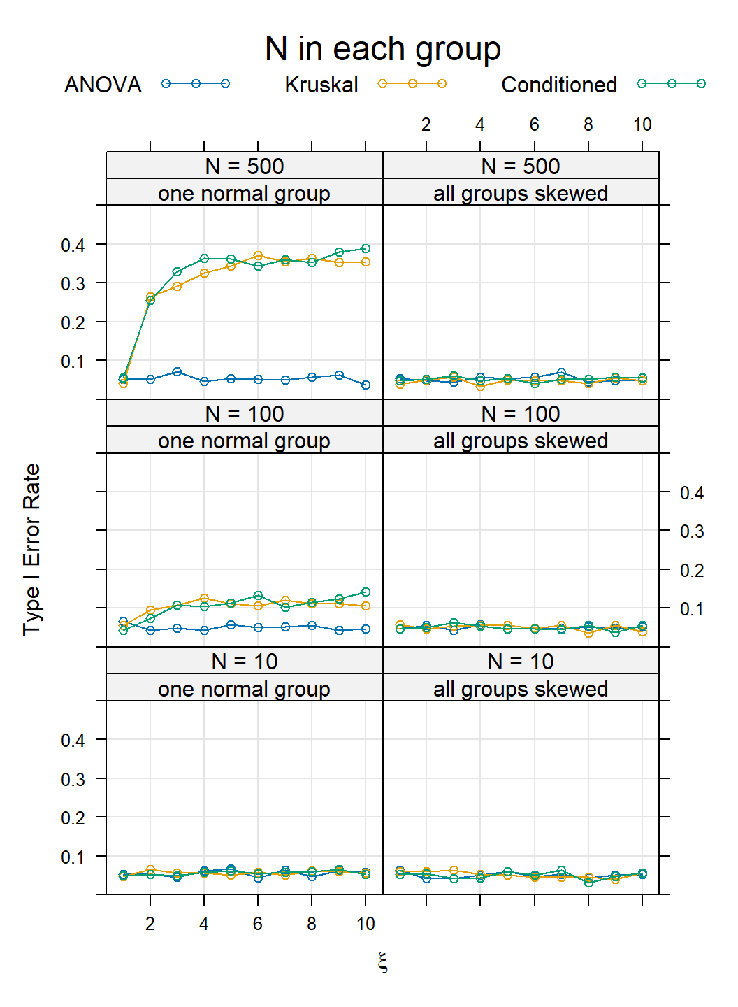
So what did we do here again? We tested for a group effect for a one-way design. We did not have an effect here, so the Type I Error Rate should not exceed \(\alpha = 0.05\), no matter what sample size we have.
I would have expected that the error rate would actually increase for the ANOVA with increasing violation of the normality assumption (that means increasing \(\xi\)). We can see that this is not the case. For the ANOVA the error rate stays at 5%, as it should. Interestingly, this is also TRUE for the Kruskal-Wallis rank sum test and for the conditioned test, when data in all groups is skewed. If data in one group is normal, then the Type I Error Rate increases for the Kruskal-Wallis rank sum test and this also implies an increase for the conditioned test. This is very pronounced for large N. I think this is very suprising and do not have an explanation for it.
But we do have an overall result: Stick to the ANOVA that you preregistered and don’t bother with testing for normality.
I only looked at one way to violate normality here. Another way could be to look at bimodal distributions or draw data from other distributions than the normal distribution. I do expect the results to look similar, but have not tried it, yet.
sessionInfo()R version 4.6.1 (2026-06-24 ucrt)
Platform: x86_64-w64-mingw32/x64
Running under: Windows 11 x64 (build 26100)
Matrix products: default
LAPACK version 3.12.1
locale:
[1] LC_COLLATE=German_Germany.utf8 LC_CTYPE=German_Germany.utf8
[3] LC_MONETARY=German_Germany.utf8 LC_NUMERIC=C
[5] LC_TIME=German_Germany.utf8
time zone: Europe/Berlin
tzcode source: internal
attached base packages:
[1] stats graphics grDevices utils datasets methods base
other attached packages:
[1] fGarch_4052.93
loaded via a namespace (and not attached):
[1] fBasics_4052.98 digest_0.6.39 fastmap_1.2.0
[4] Matrix_1.7-6 xfun_0.62 lattice_0.23-1
[7] spatial_7.3-19 knitr_1.52 gbutils_0.5.1
[10] htmltools_0.5.9 rmarkdown_2.32 Rdpack_2.6.6
[13] cli_3.6.6 cvar_0.6.1 grid_4.6.1
[16] timeDate_4052.112 compiler_4.6.1 rbibutils_2.4.1
[19] tools_4.6.1 evaluate_1.0.5 yaml_2.3.12
[22] otel_0.2.0 timeSeries_4052.112 rlang_1.3.0
[25] jsonlite_2.0.0 htmlwidgets_1.6.4