Testing a group effect when sub-groups are present
Mixed-effects models
R
Power
Author
Nora Wickelmaier
Published
September 18, 2026
Question from statistics consulting
Should I use a mixed model, wenn I have subgroups in my between groups?
The dataframe we are considering here has the following structure. We have two between groups to which we assign students from 18 different classes. Due to organizational reasons, it is easier to assign all students from one class to one condition. The assignment of the classes is random.
set.seed(1409)n <-90dat <-data.frame(id =factor(1:n),class =factor(rep(1:18, each =5)),group =factor(rep(c("ctr", "trt"), times =c(40, 50))))xtabs( ~ class + group, data = dat)
The question I was asked was, if class should be considered as a random effect in a mixed-effects model or if an independent t-test can be used to analyze these data.
This is a great example how simulation can help answering these kind of questions. Let us assume that the data generating process in this case actually is a mixed-effects model with a random intercept for class. We simulate data for one dataset and test the group effect with the following code.
# One simulated datasety <-5+0.2* lme4::dummy(dat$group) +# fixed effectsrnorm(18, mean =0, sd = .5)[dat$class] +# random intercept for classrnorm(n, mean =0, sd = .5) # random erroraggregate(y ~ group, dat, mean)
  group      trt
1   ctr 4.890459
2   trt 5.265856
# Testing the group effect# ...using mixed-effects modelsm0 <- lme4::lmer(y ~1+ (1| class), data = dat, REML =TRUE)m1 <- lme4::lmer(y ~ group + (1| class), data = dat, REML =TRUE)summary(m1)
Linear mixed model fit by REML ['lmerMod']
Formula: y ~ group + (1 | class)
   Data: dat

REML criterion at convergence: 167.2

Scaled residuals:
    Min      1Q  Median      3Q     Max
-3.1897 -0.4888 -0.0401  0.6266  2.3779

Random effects:
 Groups   Name        Variance Std.Dev.
 class    (Intercept) 0.2628   0.5127
 Residual             0.2587   0.5087
Number of obs: 90, groups:  class, 18

Fixed effects:
            Estimate Std. Error t value
(Intercept)   4.8905     0.1983  24.661
grouptrt      0.3754     0.2661   1.411

Correlation of Fixed Effects:
         (Intr)
grouptrt -0.745
# ...using an independent t-testt.test(y ~ group, data = dat, var.equal =TRUE)
    Two Sample t-test

data:  y by group
t = -2.5084, df = 88, p-value = 0.01396
alternative hypothesis: true difference in means between group ctr and group trt is not equal to 0
95 percent confidence interval:
 -0.6728038 -0.0779896
sample estimates:
mean in group ctr mean in group trt
         4.890459          5.265856
When we assume that class indeed introduces some variability into the data, then the results of the two analysis methods differ, of course. The t-test makes the assumption that all data points are indepedent, which is not the case when we have an effect of class.
Let us write a function so that we can investigate a bit more systematically.
Power simulation
pwrFun <-function(d, model, raneff_class =TRUE, nrep =1000) { pval <-replicate(nrep, {# switch between data generating moelif (raneff_class) { y <-5+ d * lme4::dummy(dat$group) +rnorm(18, mean =0, sd = .5)[dat$class] +rnorm(90, mean =0, sd = .5) } else { y <-5+ d * lme4::dummy(dat$group) +rnorm(90, mean =0, sd = .5) }# switch between analysis modelif (model =="LMM") { m0 <- lme4::lmer(y ~1+ (1| class), data = dat, REML =FALSE) m1 <- lme4::lmer(y ~ group + (1| class), data = dat, REML =FALSE)anova(m0, m1)["m1", "Pr(>Chisq)"] } elseif (model =="ttest") {t.test(y ~ group, data = dat, var.equal =TRUE)$p.value } } )# calculate powermean(pval <0.05)}pwrFun(0.2, model ="LMM", raneff_class =TRUE)
[1] 0.151
pwrFun(0.2, model ="ttest", raneff_class =TRUE)
[1] 0.404
We can see that the power to detect a group effect of 0.2 for \(\alpha = 0.05\) for the LMM and the t-test differs quite a bit when the data generating model includes a random intercept for class.
pwrFun(0.2, model ="LMM", raneff_class =FALSE)
[1] 0.415
pwrFun(0.2, model ="ttest", raneff_class =FALSE)
[1] 0.434
If we generate the data without a random intercept for class – meaning the model does not know anything of the classes – then the power for the t-test and the LMM look very similar.
Power curves
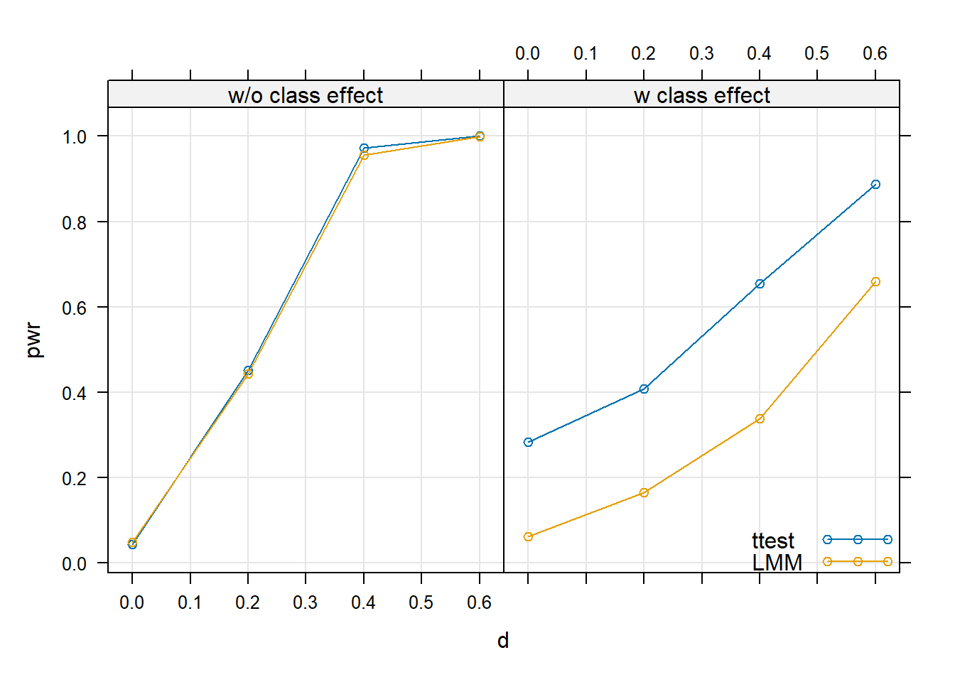
With the function above, we can now look at different combinations of the effect size and the data generating process.
The plot shows that when we generate the data without a random intercept for class, the power for different effect sizes is the same for both analysis methods. But if we generate the data with a random intercept for class, then the power for the t-test is systematically overestimated – not only when an effect is present, but also for \(d = 0\). This means we find a lot of false positives when we neglect to include class as a random intercept into the model. Hence, the question to the answer above is: “Yes, you should!”
Session info
sessionInfo()
R version 4.6.1 (2026-06-24 ucrt)
Platform: x86_64-w64-mingw32/x64
Running under: Windows 11 x64 (build 26100)

Matrix products: default
  LAPACK version 3.12.1

locale:
[1] LC_COLLATE=German_Germany.utf8  LC_CTYPE=German_Germany.utf8
[3] LC_MONETARY=German_Germany.utf8 LC_NUMERIC=C
[5] LC_TIME=German_Germany.utf8

time zone: Europe/Berlin
tzcode source: internal

attached base packages:
[1] stats     graphics  grDevices utils     datasets  methods   base

loaded via a namespace (and not attached):
 [1] lme4_2.1-0        digest_0.6.39     fastmap_1.2.0     Matrix_1.7-6
 [5] xfun_0.62         lattice_0.23-1    splines_4.6.1     knitr_1.52
 [9] htmltools_0.5.9   rmarkdown_2.32    Rdpack_2.6.6      cli_3.6.6
[13] nloptr_2.2.1      grid_4.6.1        reformulas_0.4.4  compiler_4.6.1
[17] rbibutils_2.4.1   boot_1.3-32       tools_4.6.1       nlme_3.1-171
[21] minqa_1.2.8       evaluate_1.0.5    Rcpp_1.1.2        yaml_2.3.12
[25] otel_0.2.0        rlang_1.3.0       jsonlite_2.0.0    htmlwidgets_1.6.4
[29] MASS_7.3-66