Let us look at the differences between effects and dummy coding for regression models with categorical predictors.

Model with one categorical factor

Let us simulate some data first, for \(n = 10\) subjects and a group predictor with levels ctr for the control group and trt for the treatment group.

dat <- data.frame(id    = factor(1:10),
                  group = factor(c("ctr", "trt")),
                  resp  = c(rnorm(5, mean = 1), rnorm(5)))

aggregate(resp ~ group, data = dat, FUN = mean)

  group       resp
1   ctr  0.2609670
2   trt -0.1312885

Per default R uses so-called dummy coding to represent factors. This means that the reference category (here ctr) is set to 0 and the second category is set to 1. R takes the first factor level as reference category in dummy coding.

contrasts(dat$group)

    trt
ctr   0
trt   1

You can check the default settings of your R session with

options()$contrasts

        unordered           ordered 
"contr.treatment"      "contr.poly"

The first entry "contr.treatment" indicates dummy coding.

Linear model with dummy coding

Let us now fit a simple linear regression

\[resp = \beta_0 + \beta_1 group + \varepsilon\]

with \(\varepsilon \sim N(0,\sigma_{\varepsilon})\).

(For a two-level between factor, this is equivalent to an independent t-test.)

lm1 <- lm(resp ~ group, data = dat)
summary(lm1)


Call:
lm(formula = resp ~ group, data = dat)

Residuals:
    Min      1Q  Median      3Q     Max 
-1.5820 -0.4338 -0.1752  0.6928  1.6374 

Coefficients:
            Estimate Std. Error t value Pr(>|t|)
(Intercept)   0.2610     0.4451   0.586    0.574
grouptrt     -0.3923     0.6295  -0.623    0.551

Residual standard error: 0.9953 on 8 degrees of freedom
Multiple R-squared:  0.0463,    Adjusted R-squared:  -0.07292 
F-statistic: 0.3883 on 1 and 8 DF,  p-value: 0.5505

coef(lm1)[1]    # mean ctr

(Intercept) 
   0.260967

sum(coef(lm1))  # mean trt

[1] -0.1312885

The interpretation of the parameters is straightforward: The Intercept \(\beta_0\) is the mean response in the control (here the reference) group \((\bar x_{ctr} = \beta_0)\) and \(\beta_1\) is the difference between the control and the treatment group \((\bar x_{trt} = \beta_0 + \beta_1)\).

Linear model with effects coding

Next, we will fit the same model with effects coding. Hereby, the reference group is coded as \(-1\).

contrasts(dat$group) <- "contr.sum"
contrasts(dat$group)

    [,1]
ctr    1
trt   -1

You can see that for effects coding, R takes the last factor level as reference category.

Now, let us refit the model.

lm2 <- lm(resp ~ group, dat)
summary(lm2)


Call:
lm(formula = resp ~ group, data = dat)

Residuals:
    Min      1Q  Median      3Q     Max 
-1.5820 -0.4338 -0.1752  0.6928  1.6374 

Coefficients:
            Estimate Std. Error t value Pr(>|t|)
(Intercept)  0.06484    0.31473   0.206    0.842
group1       0.19613    0.31473   0.623    0.551

Residual standard error: 0.9953 on 8 degrees of freedom
Multiple R-squared:  0.0463,    Adjusted R-squared:  -0.07292 
F-statistic: 0.3883 on 1 and 8 DF,  p-value: 0.5505

sum(coef(lm2))    # mean ctr

[1] 0.260967

-diff(coef(lm2))  # mean trt

    group1 
-0.1312885

In this model, the Intercept \(\beta_0\) is now the overall mean (often called the grand mean).

mean(dat$resp)

[1] 0.06483924

And \(\beta_1\) is the difference of the mean in group 1 (here the control group) to the overall mean and its negative value is the difference of group 1 (treatment group) to the overall mean.

Model with two categorical factors

Let us again simulate some data first. This time for \(n = 20\) subjects, a group predictor like before and an additional factor study with two levels s1 and s2.

dat <- data.frame(id    = factor(1:20),
                  group = factor(rep(c("ctr", "trt"), each = 10)),
                  study = factor(rep(c("s1", "s2"), each = 5)),
                  resp  = c(rnorm(10, mean = 1),
                            rnorm(5, mean = 0.5),
                            rnorm(5)))

aggregate(resp ~ group + study, data = dat, FUN = mean)

  group study       resp
1   ctr    s1  1.0575195
2   trt    s1  0.9622200
3   ctr    s2  1.2211857
4   trt    s2 -0.2307511

mean(dat$resp)

[1] 0.7525435

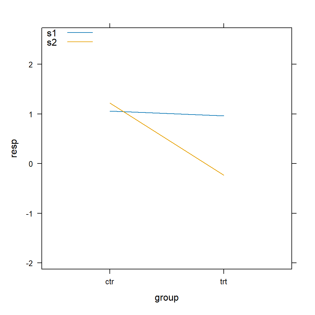
lattice::xyplot(resp ~ group, data = dat, groups = study, type = "a",
                auto.key = list(corner = c(0, 1)))

Both factors are now dummy coded, since we did not tell R to do otherwise.

contrasts(dat$group)

    trt
ctr   0
trt   1

contrasts(dat$study)

   s2
s1  0
s2  1

Linear model with dummy coding

Let us now fit regression model with an interaction term

\[resp = \beta_0 + \beta_1 group + \beta_2 study + \beta_3 (group \times study) + \varepsilon\]

with \(\varepsilon \sim N(0,\sigma_{\varepsilon})\).

(This is equivalent to a 2x2 ANOVA with two between factors.)

lm3 <- lm(resp ~ group * study, data = dat)
summary(lm3)


Call:
lm(formula = resp ~ group * study, data = dat)

Residuals:
     Min       1Q   Median       3Q      Max 
-1.59696 -0.61529  0.00399  0.56974  1.86454 

Coefficients:
                 Estimate Std. Error t value Pr(>|t|)  
(Intercept)        1.0575     0.4582   2.308   0.0347 *
grouptrt          -0.0953     0.6480  -0.147   0.8849  
studys2            0.1637     0.6480   0.253   0.8038  
grouptrt:studys2  -1.3566     0.9165  -1.480   0.1582  
---
Signif. codes:  0 '***' 0.001 '**' 0.01 '*' 0.05 '.' 0.1 ' ' 1

Residual standard error: 1.025 on 16 degrees of freedom
Multiple R-squared:  0.2826,    Adjusted R-squared:  0.1481 
F-statistic: 2.101 on 3 and 16 DF,  p-value: 0.1404

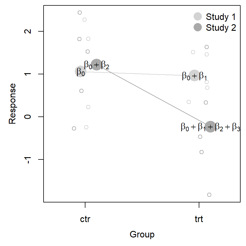
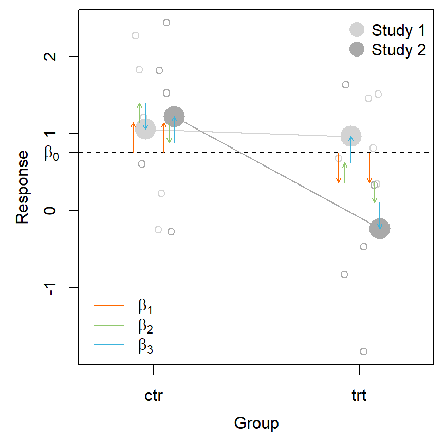
We can now reconstruct the mean values for all four groups with our parameters. The Intercept \(\beta_0\) is now the mean response in study 1 for the control group.

coef(lm3)[1]

(Intercept) 
    1.05752

coef(lm3)[1] + coef(lm3)[2]

(Intercept) 
    0.96222

coef(lm3)[1] + coef(lm3)[3]

(Intercept) 
   1.221186

coef(lm3)[1] + coef(lm3)[2] + coef(lm3)[3] + coef(lm3)[4]   # sum(coef(lm3))

(Intercept) 
 -0.2307511

With dummy coding, we can think of the dummy variables as “controlling” which parameters are entered into the mean calculations and which are not. With only categorical predictors, we get a separate equation for each of the four group means.

\[\begin{align*} resp_{11} & = \beta_0 & \text{mean s1 and crt} \\ resp_{12} & = \beta_0 + \beta_1 & \text{mean s1 and trt} \\ resp_{21} & = \beta_0 + \beta_2 & \text{mean s2 and crt} \\ resp_{22} & = \beta_0 + \beta_1 + \beta_2 + \beta_3 & \text{mean s2 und trt} \end{align*}\]

Linear model with effects coding

contrasts(dat$group) <- "contr.sum"
contrasts(dat$study) <- "contr.sum"

lm4 <- lm(resp ~ group * study, dat)
summary(lm4)


Call:
lm(formula = resp ~ group * study, data = dat)

Residuals:
     Min       1Q   Median       3Q      Max 
-1.59696 -0.61529  0.00399  0.56974  1.86454 

Coefficients:
              Estimate Std. Error t value Pr(>|t|)   
(Intercept)     0.7525     0.2291   3.285  0.00467 **
group1          0.3868     0.2291   1.688  0.11075   
study1          0.2573     0.2291   1.123  0.27796   
group1:study1  -0.3392     0.2291  -1.480  0.15822   
---
Signif. codes:  0 '***' 0.001 '**' 0.01 '*' 0.05 '.' 0.1 ' ' 1

Residual standard error: 1.025 on 16 degrees of freedom
Multiple R-squared:  0.2826,    Adjusted R-squared:  0.1481 
F-statistic: 2.101 on 3 and 16 DF,  p-value: 0.1404

coef(lm4)[1] + coef(lm4)[2] + coef(lm4)[3] + coef(lm4)[4]

(Intercept) 
    1.05752

coef(lm4)[1] - coef(lm4)[2] + coef(lm4)[3] - coef(lm4)[4]

(Intercept) 
    0.96222

coef(lm4)[1] + coef(lm4)[2] - coef(lm4)[3] - coef(lm4)[4]

(Intercept) 
   1.221186

coef(lm4)[1] - coef(lm4)[2] - coef(lm4)[3] + coef(lm4)[4]   # sum(coef(lm3))

(Intercept) 
 -0.2307511

With effects coding, all parameters are needed for calculating each of the group means. Only the signs change.

\[\begin{align*} resp_{11} & = \beta_0 + \beta_1 + \beta_2 + \beta_3 & \text{mean s1 and crt} \\ resp_{12} & = \beta_0 - \beta_1 + \beta_2 - \beta_3 & \text{mean s1 and trt} \\ resp_{21} & = \beta_0 + \beta_1 - \beta_2 - \beta_3 & \text{mean s2 and crt} \\ resp_{22} & = \beta_0 - \beta_1 - \beta_2 + \beta_3 & \text{mean s2 und trt} \end{align*}\]

Setting contrasts globally

You can also change the settings for the contrast coding globally in R.

options(contrasts = c("contr.treatment", "contr.poly"))

options()$contrasts

[1] "contr.treatment" "contr.poly"

contrasts(factor(1:3))

options(contrasts = c("contr.sum", "contr.poly"))

options()$contrasts

[1] "contr.sum"  "contr.poly"

contrasts(factor(1:3))

  [,1] [,2]
1    1    0
2    0    1
3   -1   -1

Session info

sessionInfo()

R version 4.6.1 (2026-06-24 ucrt)
Platform: x86_64-w64-mingw32/x64
Running under: Windows 11 x64 (build 26100)

Matrix products: default
  LAPACK version 3.12.1

locale:
[1] LC_COLLATE=German_Germany.utf8  LC_CTYPE=German_Germany.utf8   
[3] LC_MONETARY=German_Germany.utf8 LC_NUMERIC=C                   
[5] LC_TIME=German_Germany.utf8    

time zone: Europe/Berlin
tzcode source: internal

attached base packages:
[1] stats     graphics  grDevices utils     datasets  methods   base     

loaded via a namespace (and not attached):
 [1] htmlwidgets_1.6.4 compiler_4.6.1    fastmap_1.2.0     cli_3.6.6        
 [5] tools_4.6.1       htmltools_0.5.9   otel_0.2.0        yaml_2.3.12      
 [9] rmarkdown_2.32    grid_4.6.1        knitr_1.52        jsonlite_2.0.0   
[13] xfun_0.62         digest_0.6.39     rlang_1.3.0       lattice_0.23-1   
[17] evaluate_1.0.5